Changing causal structures: Simpson’s Paradox 2

This is the second in a series of posts which discusses the causality and Simpson’s Paradox. For the 1st part see Causality, Confounding, and Simpson’s Paradox 1 where, there is not one (gender) but two causal factors (gender and difficulty level per department) that influence the admission rates. Being female is a positive influencer in each department but applying to humanities is a strong negative influencer. As men applied more to engineering their negative influencer (gender) was overwhelmed by their positive influence of department choice (engineering). Bickel et. al. (1975) noted this paradox, and provided this explanation. This explanation is just a conjecture about the causal factors which affect admissions rates. It is possible that taking into account other causal factors (like GPA) could lead to entirely different analysis of exactly the same data. For example, suppose admissions policies at ENG and HUM are only based on GPA, but HUM is more difficult to get into:

	Admit Percent
Grade	ENG	ENG
A	90%	60%
B	70%	30%
C	50%	10%

If female applicant pool has better grades (i.e. 60% A’s, 30% B’s and 10% C’s) while male applicant pool has significantly lower GPA’s (10% A’s, 30% B’s and 60% C’s), then exactly same admission patterns will be observed. The original data appears to show gender bias – females are preferred. But deeper analysis reveals that there is no discrimination by gender. The admissions criteria are the same for both genders, but more females get in because they have higher grades. Now the causal question here would be why better male applicants do not apply to Berkeley while better female applicants do? Answer may lie in availability of a good all-male university which is not available for females. Or, one could construct examples where females are better at English and males are better at math, and this provides the causal explanation. Now these answers to the WHY questions do not come from numbers; we are speculating about unobserved, real structural factors. This is the central point of the article: numbers do not contain causal information, whereas understanding the numbers needs causal understanding, which only comes from qualitative kinds of knowledge about deeper structures of reality. Current econometric practices are deeply flawed because they can only be used to describe correlations among observations, and do not take causal information into consideration. Even worse, they encourage intellectual laziness among students, who are taught to believe that running a regression yields reliable results without any considerations of causal structures.

As noted by Pearl (2018) and Hoover (2004), a major obstacle to development of causal thinking has been the lack of mathematical notation to express causality. In particular, the “equal sign” in a regression model (C= a + bY) does not give us a clue that Y is a cause of C, and encourages the mistaken algebra that Y=(C/b)-(a/b), which is not correct as a causal equation. One of the critical factors in the development of understanding about causality has been the development of a natural language to express causal relationships. This is the language of path diagrams, which we now introduce. The causal structure of the explanation given by Bickel et. al. (1975) for Simpson’s Paradox in Berkeley admissions can be depicted in the following path diagram.

Causal Map # 1(Bickel)

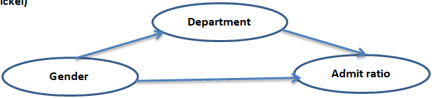
Here gender affects both the choice of department and admit ratio. Department also affects admit ratio. The causal path diagram is crucial in determining exogeneity and endogeneity. These are key concepts used in Econometrics, but they remain confusing because they cannot be defined correctly without understanding causality. To understand this better, suppose we want to study how choice of department affects the admit ratios. The path diagram above shows that Gender influences both Department choice and the admit ratio, but it is NOT influenced by either of these variables. This makes Gender exogenous. To be more precise: When we are studying the effect of department on the admission ratio, gender is exogenous because it is not causally influenced by either of the two variables under study. Statisticians say that Gender is a confounding variable, but are equally confused about the meaning of confounding, because understanding it requires causality. To solve this problem of confounding, we must CONDITION on gender. In the language of econometrics, exogeneity means that we can condition on this variable, treating it as constant. Holding gender constant — i.e. separately calculating admit rates for both genders – allows us to calculate the effect of department choice on admit ratio, while preventing the confounding variable from changing, so as to eliminate its effects.

However, if we want to calculate the effect of gender on admit ratio, the causal structure is different. Department choice is affected by Gender, and so this cannot be taken as an exogenous variable for this analysis. We cannot condition on the department to derive effect of gender on admit rate. A different way of thinking about the situation is required. The causal diagram shows that Gender affects admit ratio via two pathways. One is a direct effect, and the second is an indirect effect via department choice. Both effects must be considered to derive the total effect of gender on admit ratio. Say for example John and Jane apply to Berkeley. Suppose we do not know their department choice, and wish to calculate their probability of being admitted. Then we should use their respective overall admit ratios, 56% and 44% for calculating their chance of admission. Following tree diagrams trace the probabilities of various outcomes and paths.

Figure # 1: Female Admit Probabilities Tree Diagram

Figure # 2: Female Admit Probabilities Tree Diagram

Only 10% females choose Engineering, where they have 80% chances of admission and 90% females choose Humanities but with only 40% chances of admission. Applying this past data, we can estimate that Jane will apply to HUM with 90% probability and to ENG with 10% probability. Using the admit rates for females in ENG and HUM, we can compute her chances of getting admission as: 90% *40% + 10%*80% = 36% + 8% = 44%. This calculation is valid under the assumption that the past history of admissions applies to Jane – she is not differentiated from the typical female applicant in ways which would make the history irrelevant.

For John, we have the same diagram, but the probabilities are different at each branch of the tree for males.

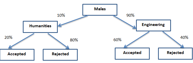
Figure # 3: Male Admit Probabilities Tree Diagram

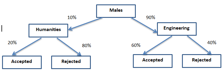
John has a 10% chance of applying to HUM and a 90% chance of applying to ENG. In the two departments, his admit probabilities are 20% and 60% respectively, so his overall admit probability is 10% *20% + 90%*60% = 2% + 54% = 56%

These calculations show that the probability for females to get into Berkeley is only 44%, while the probability for males is 56%. These aggregate numbers correctly reflect overall admit probabilities categorized by Gender (without conditioning on the Department). On the other hand, if the department choices for Jane and John are known, then entirely different probabilities would apply. The question of when we should condition, and when we should not, depends entirely on the research question we are trying to answer. There is considerable confusion about this matter mainly because there is no way to explicitly take into account causal information in conventional statistical and econometric analysis.

For other parts in sequence see:

Causality, Confounding, and Simpson’s Paradox 1 ,

Policy depends upon unobservable causal relations: Simpson’s Paradox 3,

Baseball scores: Overall Average or Stratified?: Simpson’s Paradox 4,

Effect of Drugs on Recovery 1: Simpson’s Paradox 5 &

Effect of Drugs on Recovery 2: Simpson’s Paradox 5 —- continued.